What happens when a stock joins an index? An Analysis with Python
- Nikhil Adithyan
- Oct 1, 2024
- 10 min read
Digging deep into the aftermath of stocks’ inclusion into an index

Every trader, even during his baby steps, knows about SP500, and that this is like the benchmark of how the stock market moved on a specific day. But let’s talk just a bit about theory:
What Are Stock Market Indexes and How Are They Composed?
A stock market index tracks a specific group of stocks to reflect overall market trends. For example, the S&P 500 includes 500 of the largest U.S. companies, such as Apple and Microsoft. Investors often use these indexes to compare their portfolio’s performance against the broader market.
Each index has constituents, or stocks, that meet specific criteria. In the S&P 500, only large-cap companies like Tesla or Alphabet are included. These companies must meet standards for market size and liquidity, and the list is updated regularly to reflect market changes.
The weight of each stock in an index is often based on market capitalization. This means larger companies, like Amazon, have more influence on the index’s performance. In the S&P 500, a market-cap-weighted system ensures that bigger companies drive more of the index movement.
How Index Inclusion Impacts Traders
When a stock is added to an index like the S&P 500, its price often rises due to increased demand from funds tracking the index. This “index effect” creates opportunities for traders. For instance, when Tesla joined the S&P 500, traders anticipated a price jump and acted accordingly.
Traders can also predict index changes by analyzing the selection criteria. Knowing which companies might be added or removed helps traders take advantage of stock price movements. For example, when a smaller company gets added, traders might buy shares early to benefit from the price increase caused by its inclusion in the index.
But enough about theory. Let’s see what actually happens in practice.
What will we try to achieve in this article:
Using the Indices Historical Constituents Data API from EODHD, we will create a dataset of all the entries of stocks in the relevant indexes
We will get the end-of-day candles of those shares and calculate the metrics needed for our analysis
we will analyze the reaction of the stocks before and after their inclusion in the index
Let’s code!
First, we will do the necessary imports, set our EODHD API Key, and download the list of supported indices
import pandas as pd
import matplotlib.pyplot as plt
import requests
import itertools
import json
import io

token = 'YOUR API KEY'

url = f'https://eodhd.com/api/mp/unicornbay/spglobal/list'
querystring = {"api_token":token,"fmt":"json"}
index_list = requests.get(url, params = querystring).json()
df = pd.DataFrame(index_list)

df
Take some time to get familiar with the dataset. You will see that there are more than 100 indices from all over the world, but of course, the majority are from the US.

With the use of the above list, we will be able to query again the EODHD API and get the current constituents, as well as the historical entries and exits from the index of the last 12 years.
Let’s see for example the S&P 500:
url = f'https://eodhd.com/api/mp/unicornbay/spglobal/comp/GSPC.INDX'
querystring = {"api_token":token,"fmt":"json"}
data = requests.get(url, params=querystring).json()
df_comp = pd.DataFrame.from_dict(data['Components'], orient='index')

df_comp

You can see from the above, that the first part of the response (components) provides the current constituents, Sector, Industry, and their weight on the index.
df_hist = pd.DataFrame.from_dict(data['HistoricalTickerComponents'], orient='index')

df_hist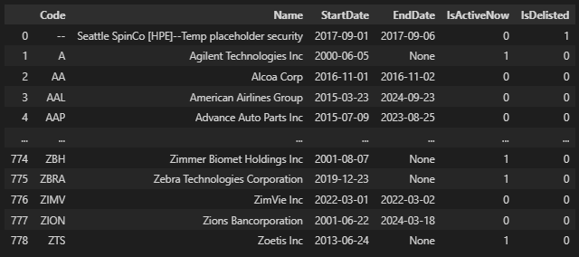
The second part of the response provides the historical entries and exists of stocks in the index, together with if they are active now or delisted.
Now we will create our dataset that we will base our full investigation on. For that reason, we will iterate through the list of indices (index_list) that we got before, gather the current components of them, as well the historical entries, and concatenate into one dataframe that will keep both information.
df_list = []

for idx in index_list:
    try:
        url = f'https://eodhd.com/api/mp/unicornbay/spglobal/comp/{idx["ID"]}'
        querystring = {"api_token":token,"fmt":"json"}
        data = requests.get(url, params=querystring).json()
        if data['Components'] != {}:
            df_comp = pd.DataFrame.from_dict(data['Components'], orient='index')
            df_comp.set_index('Code', inplace=True)
            df_hist = pd.DataFrame.from_dict(data['HistoricalTickerComponents'], orient='index')
            df_hist.set_index('Code', inplace=True)
        else:
            continue
        df_merged = pd.concat([df_comp[['Exchange', 'Name', 'Sector', 'Industry', 'Weight']], df_hist[['StartDate', 'EndDate', 'IsActiveNow', 'IsDelisted']]], axis=1)
        df_merged['index'] = idx['ID']
        path = 'C:/Users/nikhi/OneDrive/Desktop/Scriptonomy/EODHD/Stock Indices entry/'
        df_merged.to_csv(path+f'index_data/{idx["ID"]}_merged.csv')
        df_list.append(df_merged)

    except Exception as e:
        print(e)

df_concat_list = pd.concat(df_list, axis=0)
df_concat_list['StartDate'] = pd.to_datetime(df_concat_list['StartDate'], errors='coerce')
df_concat_list= df_concat_list.reset_index()

df_concat_list
Unfortunately, the part of the historic entries of the API, does not provide the name, sector, and industry of the stock. But this we will need later on for the analysis. So we should fix it.
For that reason we will need to call for each stock in the dataframe, the EODHD API for fundamentals that will provide us with this information:
# Keep track of already updated 'Code' to avoid redundant API calls
updated_codes = {}

# Iterate over rows with missing 'Name' and update all rows with the same 'Code'
for index, row in df_concat_list.iterrows():
    code = row['Code']

    if code not in updated_codes:
        # Call the API with 'code' and get 'Name', 'Sector', and 'Industry' (API logic to be added)
        try:
            url = f'https://eodhd.com/api/fundamentals/{code}'
            querystring = {"api_token":token,"fmt":"json"}
            data = requests.get(url, params=querystring).json()

            name = data['General']['Name']
            sector = data['General']['Sector']
            industry = data['General']['Industry']
        except Exception as e:
            print(e)

        # Update all rows with the same 'Code'
        df_concat_list.loc[df_concat_list['Code'] == code, ['Name', 'Sector', 'Industry']] = [name, sector, industry]

        # Store the updated 'Code' to skip redundant API calls
        updated_codes[code] = True

df_concat_list
With a closer look at the dataframe we can understand that the sector some times it is mentioned in a different way. For example, if you run the above, you will be able to see that we have 3 different names for the sector “Financials” and these are Financial Services, Financials, and *Financial.
Now it is time for some standardisation. We will use the Global Industry Classification Standard (GICS). Without getting into a lot of details, we will run the below code to fix the issue.
# apply the sector cleaning mapping based on the official GICS sectors
sector_mapping = {
    'Utilities': 'Utilities',
    'Financial Services': 'Financials',
    'Financials': 'Financials',
    'Financial': 'Financials',
    'Industrials': 'Industrials',
    'Industrial Goods': 'Industrials',
    'Consumer Cyclical': 'Consumer Discretionary',
    'Consumer Discretionary': 'Consumer Discretionary',
    'Consumer Defensive': 'Consumer Staples',
    'Consumer Goods': 'Consumer Staples',
    'Consumer Non-Cyclicals': 'Consumer Staples',
    'Healthcare': 'Health Care',
    'Energy': 'Energy',
    'Communication Services': 'Communication Services',
    'Technology': 'Information Technology',
    'Information Technology': 'Information Technology',
    'Basic Materials': 'Materials',
    'Materials': 'Materials',
    'Real Estate': 'Real Estate',
    'Services': 'Other',  # Assuming 'Services' is too broad
    'Other': 'Other',  # Keeping 'Other' as is
    'Pharmaceuticals': 'Health Care',  # Pharmaceuticals likely falls under Health Care
}

# Apply the mapping to clean up the 'Sector' column
df_concat_list['Sector'] = df_concat_list['Sector'].map(sector_mapping)
Let’s have now our first plot. Since there are quite a few indexes, we will focus on the S&P ones from 100, 400,500,600,900,1000,1500.
# List of indices to focus on
sp_indices = ['SP1500.INDX', 'SML.INDX', 'OEX.INDX', 'GSPC.INDX', 'SP900.INDX', 'SP1000.INDX', 'MID.INDX']

# Create a mapping of index codes to business names
index_name_map = {
    'SP1500.INDX': 'S&P Composite 1500',
    'SML.INDX': 'S&P 600',
    'OEX.INDX': 'S&P 100',
    'GSPC.INDX': 'S&P 500',
    'SP900.INDX': 'S&P 900',
    'SP1000.INDX': 'S&P 1000',
    'MID.INDX':'S&P 400'
}

# Group by sector and index to calculate total weight for each in the respective indices
sector_industry_trends = df_concat_list.groupby(['index', 'Sector', 'Industry'])['Weight'].sum().reset_index()

# Filter the dataset to include only the corrected S&P indices
sp_sector_trends_corrected = sector_industry_trends[sector_industry_trends['index'].isin(sp_indices)]

# Group by index and sector to calculate the total weight for each sector in these indices
sp_sector_summary_corrected = sp_sector_trends_corrected.groupby(['index', 'Sector'])['Weight'].sum().reset_index()

# Plot: Sector dominance for the corrected S&P indices
plt.figure(figsize=(10, 6))
for idx in sp_sector_summary_corrected['index'].unique():
    subset = sp_sector_summary_corrected[sp_sector_summary_corrected['index'] == idx]
    # Use the business name from the mapping
    plt.bar(subset['Sector'], subset['Weight'], label=index_name_map[idx])

plt.xticks(rotation=45, ha='right')
plt.ylabel('Total Weight')
plt.title('Sector Dominance in Selected S&P Indices')
plt.legend(title='Index')
plt.tight_layout()
plt.show()

You will see above that (as expected to be fair) the Information Technology sector is dominating the plot. Industrials, Financials, and Consumer Discretionary are the following.
Let’s check the reaction
Now it is time to get to the actual analysis. Using the same dataframe (but for the last 10 years), we will update it with the below data points:
Check at which point of the trend is the stock. We will calculate how far is above or below the MA50, MA100, and MA200, the current price
We will calculate for the next 3, 6, and 12 months, what was the price change from the day of inclusion in the index
Also, we should check how the stock price was trading after the inclusion. For that reason, we will calculate how many times the price was above the MA50, MA100, and MA200 for 3, 6, and 12 months
Let’s get those numbers:
# Get the rows that have a start date and also are from the last 10 years
df_inclusion_reaction = df_concat_list[(df_concat_list['StartDate'].notna()) & (df_concat_list['StartDate'] > '2014-01-01') & (df_concat_list['StartDate'] < '2023-09-25')]

list_of_time_horison_months = [3,6,12]
list_of_MA_periods = [50,100,200]

for index, row in df_inclusion_reaction.iterrows():
        try:
            stock = row['Code']
            from_date = pd.to_datetime(row['StartDate'])

            # calculate till date
            list_till_date = []
            for th in list_of_time_horison_months:
                list_till_date.append(from_date + pd.DateOffset(months=th))

            # get ohlc
            url = f'https://eodhd.com/api/eod/{stock}'
            querystring = {"api_token":token,"fmt":"csv"}
            response = requests.get(url, params=querystring)
            eod_df = pd.read_csv(io.StringIO(response.text))

            eod_df['Date'] = pd.to_datetime(eod_df['Date'])
            eod_df.set_index('Date', inplace=True)

            # calculate MAs
            for ma in list_of_MA_periods:
                eod_df[f'MA_{ma}'] = eod_df['Adjusted_close'].rolling(window=ma).mean()

            # Calculate current status of MA
            for ma in list_of_MA_periods:
                filtered_df = eod_df[(eod_df.index >= from_date)]
                pct_from_MA = ((filtered_df[f'Adjusted_close'].iloc[0] - filtered_df[f'MA_{ma}'].iloc[0]) / filtered_df[f'MA_{ma}'].iloc[0]) * 100
                # update the result
                df_inclusion_reaction.loc[index, f'Pct_from_MA_{ma}_at_StartDate'] = pct_from_MA

            # calculate profits and losses depending on the time horizon
            for ith in range(len(list_of_time_horison_months)):
                filtered_df = eod_df[(eod_df.index >= from_date) & (eod_df.index < list_till_date[ith])]
                # calculate the diff in price from from date to till date
                from_price = filtered_df.iloc[0]['Adjusted_close']
                till_price = filtered_df.iloc[-1]['Adjusted_close']
                diff_pct = ((till_price - from_price) / from_price) * 100
                # update the result
                df_inclusion_reaction.loc[index, f'PnL_{list_of_time_horison_months[ith]}'] = diff_pct

            # calculate percentage of above MA after into the time horizon
            for ith, ima in itertools.product(range(len(list_of_time_horison_months)), range(len(list_of_MA_periods))):
                filtered_df = eod_df[(eod_df.index >= from_date) & (eod_df.index < list_till_date[ith])]
                # Count how many times the closing price is greater than the 200-day MA
                count_above = (filtered_df['Adjusted_close'] > filtered_df[f'MA_{list_of_MA_periods[ima]}']).sum()
                total_observations = len(filtered_df)
                percentage_above_MA = (count_above / total_observations) * 100
                # update the result
                df_inclusion_reaction.loc[index, f'Above_MA_{list_of_MA_periods[ima]}_for_{list_of_time_horison_months[ith]}_months'] = percentage_above_MA

        except Exception as e:
            print(e)

df_inclusion_reaction
Now the best is to get some preliminary information on the data points that we have calculated using a histogram. Keep the below function in your code snippets, it is very handy ;)
columns_to_plot = ['PnL_3', 'PnL_6', 'PnL_12',
       'Above_MA_50_for_3_months', 'Above_MA_100_for_3_months',
       'Above_MA_200_for_3_months', 'Above_MA_50_for_6_months',
       'Above_MA_100_for_6_months', 'Above_MA_200_for_6_months',
       'Above_MA_50_for_12_months', 'Above_MA_100_for_12_months',
       'Above_MA_200_for_12_months']

def plot_histograms(df, columns, bins=10, nrows=None, ncols=None, std=0):
    num_columns = len(columns)

    # Set default nrows and ncols if not provided
    if not nrows or not ncols:
        ncols = math.ceil(math.sqrt(num_columns))  # Set ncols to the square root of the number of columns
        nrows = math.ceil(num_columns / ncols)     # Set nrows based on the total number of plots and ncols

    # Set up the figure and subplots
    fig, axes = plt.subplots(nrows=nrows, ncols=ncols, figsize=(7 * ncols, 3 * nrows))

    # Flatten the axes array if it's multidimensional
    if isinstance(axes, np.ndarray):
        axes = axes.flatten()
    else:
        axes = [axes]  # Handle single subplot case

    for i, column in enumerate(columns):
        if column in df.columns:
            # Drop NaN values for plotting
            data = df[column].dropna()

            # Outlier removal based on standard deviation
            if std > 0:
                mean = data.mean()
                std_dev = data.std()
                data = data[(data >= mean - std * std_dev) & (data <= mean + std * std_dev)]

            # Plot the histogram
            axes[i].hist(data, bins=bins, edgecolor='black')

            # Set titles and labels
            axes[i].set_title(f'Histogram of {column}')
            axes[i].set_xlabel(column)
            axes[i].set_ylabel('Frequency')
        else:
            print(f"Column {column} not found in DataFrame")

    # Hide unused subplots
    for j in range(len(columns), len(axes)):
        axes[j].set_visible(False)  # Hide the unused subplots instead of deleting them

    # Adjust layout to avoid overlapping plots
    plt.tight_layout()

    # Show the plot
    plt.show()

plot_histograms(df_inclusion_reaction, columns_to_plot, bins=20, ncols=3, nrows=5,  std=2)

The top 3 are the histograms of the price difference, between the inclusion day, till 3,6 and 12 months after. We cannot see any trend. The dataset is completely balanced, with the mean close to zero (no change in the price).
The rest of the histograms are all combinations of trending for 3, 6, and 12 months, combined with MA50, MA100 and MA200. I will focus on 2 of them:
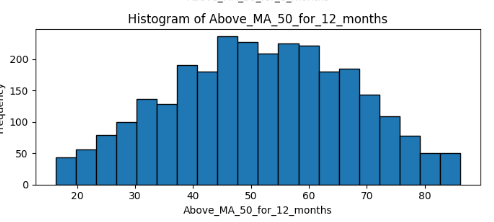
The fastest MA (50) combined with a long period (12 months) looks balanced on the 50%. This means that the MA is crossing more frequently the price, and the longest period seems to normalize the distribution. There is no surprise here. However:
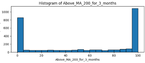
The slowest MA (200) with a short period has the majority of data points to 0 and 100. Practically this means that the stock that enters an index usually remains on the same long trend (upwards or downwards) at least for 3 months.
Now we will try to put the previous trend in the game! But first let’s see what is the possibility of a stock to be having a positive PnL after its inclusion in the index
# Filter columns related to PnL
pnl_columns = ['PnL_3', 'PnL_6', 'PnL_12']

# Calculate the percentage of positive and negative values for each PnL column
positive_negative_ratios = {}
for col in pnl_columns:
    positive_negative_ratios[col] = [
        (df_inclusion_reaction[col] > 0).sum(),  # Count of positive values
        (df_inclusion_reaction[col] <= 0).sum()   # Count of negative values
    ]

# Plot pie charts for each PnL column as subplots
fig, axes = plt.subplots(1, 3, figsize=(18, 6))

for i, col in enumerate(pnl_columns):
    axes[i].pie(
        positive_negative_ratios[col],
        labels=['Positive', 'Negative'],
        autopct='%1.1f%%',
        startangle=90
    )
    axes[i].set_title(f'{col} Distribution')

plt.tight_layout()
plt.show()

The results are 50–50, like a coin toss. Even if we filter to the accounts that were already trading upwards, we will not see significant improvement as we will see in the below pie charts.
# Filter the dataframe for stocks that were trending up (Pct_from_MA_200_at_StartDate > 0)
df_trending_up = df_inclusion_reaction[df_inclusion_reaction['Pct_from_MA_200_at_StartDate'] > 0]

# Calculate the percentage of positive and negative values for each PnL column for trending stocks
positive_negative_ratios_trending = {}
for col in pnl_columns:
    positive_negative_ratios_trending[col] = [
        (df_trending_up[col] > 0).sum(),  # Count of positive values
        (df_trending_up[col] <= 0).sum()   # Count of negative values
    ]

# Plot pie charts for each PnL column as subplots for trending stocks
fig, axes = plt.subplots(1, 3, figsize=(18, 6))

for i, col in enumerate(pnl_columns):
    axes[i].pie(
        positive_negative_ratios_trending[col],
        labels=['Positive', 'Negative'],
        autopct='%1.1f%%',
        startangle=90
    )
    axes[i].set_title(f'{col} Distribution (Trending Up)')

plt.tight_layout()
plt.show()

Conclusion
The inclusion of a stock in an index is a big milestone for the company. However, the significance of it does not reflect the data that we saw. Let’s try to summarize our findings:
Index Inclusion and Current Trend: The inclusion of a stock in a major index alone does not necessarily predict the future trend of that stock. While inclusion can lead to increased demand due to index funds buying the stock, the actual price trend depends on many other factors such as overall market sentiment, investor psychology, and macroeconomic conditions. The mixed results observed in your analysis demonstrate that inclusion isn’t a reliable predictor of short-term or long-term price movement.
Inclusion as a Fundamental Indication: Inclusion in an index is, by default, a positive indicator from a fundamental perspective. It generally implies that the company meets certain size, liquidity, and stability requirements, often reflecting good overall health. However, being fundamentally sound doesn’t always translate into immediate price appreciation, especially in the short term, as market participants may have already priced in the news or other market dynamics could overshadow the effect of the inclusion.
With that being said, you’ve reached the end of the article. I hope you enjoyed the article and most of all, that this was food for thought, to accompany your trading journey. Thank you very much for your time.
Disclaimer: While we explore the exciting world of investing in this article, it’s crucial to note that the information provided is for educational purposes only. I’m not a financial advisor, and the content here doesn’t constitute financial advice. Always do your research and consider consulting with a professional before making any investment decisions.
Comments