A very interesting analysis with Python

Earnings announcements are one of the most anticipated events in the financial markets. Every quarter, companies reveal their financial performance, and these reports can significantly impact stock prices, especially when there’s a large discrepancy between the expected and actual results.
What you should expect
During the article, we will try to answer:
How do stock prices behave in the days before and after earnings reports?
How do stocks react to earnings surprises (both positive and negative)?
How does pre-announcement increased volume or volatility affect the after-announcement price?
Are certain sectors more predictable than others?
How are we going to do that
With the use of the EODHD Fundamental API and Python, we are going to get the earning results of 100 S&P 500 stocks from various sectors, for the last 10 years, and:
Identify the price action of 10 days, or 1 month before and after the announcement
Calculate some metrics like existing trends during the announcement, if analysts were estimating more than the previous EPS, etc
Identify consistencies in the results, like continuous growth
The most important metrics that you should have in mind are EPS and PE:
Earnings Per Share (EPS) measures a company’s profitability by dividing net income by the number of outstanding shares. It indicates how much profit each share of stock generates for shareholders.
The Price-to-Earnings Trailing Twelve Months (P/E TTM) ratio measures a company’s stock price relative to its Earnings Per Share (EPS) over the past 12 months. It reflects historical profitability and current market valuation.
Let’s prepare the data
To prepare the data we are going to write a function, where we will be passing as a parameter the stock ticker, and it will return a dataframe with all the calculated metrics. In the end, we will have a dataframe with all the 100 stocks earning reports of the last 10 years.
import requests
import pandas as pd
import matplotlib.pyplot as plt
import numpy as np

token = 'YOUR API KEY'

def prepare_df(stock, sector, token):

    url = f'https://eodhd.com/api/fundamentals/{stock}'
    querystring = {"api_token":token,"fmt":"json"}
    data = requests.get(url, params=querystring).json()
    earnings_data = data['Earnings']['History']
    df = pd.DataFrame.from_dict(earnings_data, orient='index')
    df.dropna(inplace=True)

    df['stock'] = stock
    df['sector'] = sector

    # calculate the yearly trailing eps that is the sum of the last 4 quarter eps
    df['EPS_TTM'] = df['epsActual'][::-1].rolling(window=4).sum()[::-1]

    from_date  = df['date'].min()

    url = f'https://eodhd.com/api/eod/{stock}'
    querystring = {"api_token":token,"fmt":"json","from":from_date}
    stock_eod = requests.get(url, params=querystring).json()
    eod_df = pd.DataFrame(stock_eod)

    # calculate the last months average volume
    eod_df['avg_volume'] = eod_df['volume'].rolling(window=22).mean().apply(lambda x: int(x) if not pd.isna(x) else np.nan)
    eod_df['avg_volume_next_5'] = eod_df['volume'].shift(-5).rolling(window=5).mean().apply(lambda x: int(x) if not pd.isna(x) else np.nan)
    eod_df['avg_volume_before_5'] = eod_df['volume'].rolling(window=5).mean().apply(lambda x: int(x) if not pd.isna(x) else np.nan)
    # eod_df['volume_change_pct_after'] = ((eod_df['avg_volume_next_5'] - eod_df['avg_volume']) / eod_df['avg_volume'])*100
    eod_df['volume_change_pct_before'] = ((eod_df['avg_volume_before_5'] - eod_df['avg_volume']) / eod_df['avg_volume'])*100

    # calculate the montly rolling volatility
    eod_df['Returns'] = eod_df['adjusted_close'].pct_change()
    eod_df['Rolling_Volatility_22'] = eod_df['Returns'].rolling(window=22).std() * (252**0.5)
    eod_df['Rolling_Volatility_5'] = eod_df['Returns'].rolling(window=5).std() * (252**0.5)
    # eod_df['Rolling_Volatility_next_5'] = eod_df['Returns'].shift(-5).rolling(window=5).std() * (252**0.5)
    # eod_df['volatility_change2_after_pct'] = ((eod_df['Rolling_Volatility_next_5'] - eod_df['Rolling_Volatility_5']) / eod_df['Rolling_Volatility_5'])*100
    eod_df['volatility_change_before_pct'] = ((eod_df['Rolling_Volatility_5'] - eod_df['Rolling_Volatility_22']) / eod_df['Rolling_Volatility_22'])*100

    # calculate diff from previous 10 or 22 days
    eod_df['diff_10_before_pct'] = (eod_df['adjusted_close'] - eod_df['adjusted_close'].shift(10))/eod_df['adjusted_close'].shift(10) * 100
    eod_df['diff_22_before_pct'] = (eod_df['adjusted_close'] - eod_df['adjusted_close'].shift(22))/eod_df['adjusted_close'].shift(22) * 100

    # calculate diff from after 10 or 22 days
    eod_df['diff_10_after_pct'] = (eod_df['adjusted_close'].shift(-10) - eod_df['adjusted_close'] )/eod_df['adjusted_close'] * 100
    eod_df['diff_22_after_pct'] = (eod_df['adjusted_close'].shift(-22)  - eod_df['adjusted_close'])/eod_df['adjusted_close'] * 100

    # put if the date is a reporting date
    eod_df['ReportingDate'] = eod_df['date'].isin(df['reportDate'])


    benchmark_ticker = 'SPY'
    url = f'https://eodhd.com/api/eod/{benchmark_ticker}'
    querystring = {"api_token":token,"fmt":"json","from":from_date}
    benchmark_eod = requests.get(url, params=querystring).json()
    eod_benchmark_df = pd.DataFrame(benchmark_eod)

    # calculate diff from previous 10 or 22 days
    eod_benchmark_df['diff_10_before_benchmark_pct'] = (eod_benchmark_df['adjusted_close'] - eod_benchmark_df['adjusted_close'].shift(10))/eod_benchmark_df['adjusted_close'].shift(10) * 100
    eod_benchmark_df['diff_22_before_benchmark_pct'] = (eod_benchmark_df['adjusted_close'] - eod_benchmark_df['adjusted_close'].shift(22))/eod_benchmark_df['adjusted_close'].shift(22) * 100

    # calculate diff from after 10 or 22 days
    eod_benchmark_df['diff_10_after_benchmark_pct'] = (eod_benchmark_df['adjusted_close'].shift(-10) - eod_benchmark_df['adjusted_close'])/eod_benchmark_df['adjusted_close'] * 100
    eod_benchmark_df['diff_22_after_benchmark_pct'] = (eod_benchmark_df['adjusted_close'].shift(-22) - eod_benchmark_df['adjusted_close'])/eod_benchmark_df['adjusted_close'] * 100

    df['reportDate'] = pd.to_datetime(df['reportDate'])
    eod_df['date'] = pd.to_datetime(eod_df['date'])
    eod_benchmark_df['date'] = pd.to_datetime(eod_df['date'])

    # df['trend'] = None
    df['close_before_report'] = None
    df['close_before_report'] = df['close_before_report'].astype(float)
    df['open_after_report'] = None
    df['open_after_report'] = df['open_after_report'].astype(float)
    df['close_benchmark'] = None
    df['close_benchmark'] = df['close_benchmark'].astype(float)
    df['open_benchmark'] = None
    df['open_benchmark'] = df['open_benchmark'].astype(float)

    for index, row in df.iterrows():
        report_date = row['reportDate']

        # Get the day before the report date and the day after
        day_before = report_date - pd.Timedelta(days=1)
        day_after = report_date + pd.Timedelta(days=1)

        # move fields from reporting's day to the earnings dataframe
        eod_reporting_date = eod_df[eod_df['date'] <= report_date].sort_values(by='date', ascending=False).head(1)
        if not eod_reporting_date.empty:
            df.at[index, 'diff_10_before_pct'] = eod_reporting_date['diff_10_before_pct'].values[0]
            df.at[index, 'diff_22_before_pct'] = eod_reporting_date['diff_22_before_pct'].values[0]
            df.at[index, 'diff_10_after_pct'] = eod_reporting_date['diff_10_after_pct'].values[0]
            df.at[index, 'diff_22_after_pct'] = eod_reporting_date['diff_22_after_pct'].values[0]
            df.at[index, 'volume_change_pct_before'] = eod_reporting_date['volume_change_pct_before'].values[0]
            df.at[index, 'volatility_change_before_pct'] = eod_reporting_date['volatility_change_before_pct'].values[0]

        # move fields from reporting's day of benchamrk to the earnings dataframe
        eod_reporting_date_benchmark = eod_benchmark_df[eod_benchmark_df['date'] <= report_date].sort_values(by='date', ascending=False).head(1)
        if not eod_reporting_date_benchmark.empty:
            df.at[index, 'diff_10_before_benchmark_pct'] = eod_reporting_date_benchmark['diff_10_before_benchmark_pct'].values[0]
            df.at[index, 'diff_22_before_benchmark_pct'] = eod_reporting_date_benchmark['diff_22_before_benchmark_pct'].values[0]
            df.at[index, 'diff_10_after_benchmark_pct'] = eod_reporting_date_benchmark['diff_10_after_benchmark_pct'].values[0]
            df.at[index, 'diff_22_after_benchmark_pct'] = eod_reporting_date_benchmark['diff_22_after_benchmark_pct'].values[0]


        # Find the closest date before or equal to the day_before
        close_before = eod_df[eod_df['date'] <= day_before].sort_values(by='date', ascending=False).head(1)['adjusted_close']
        if not close_before.empty:
            df.at[index, 'close_before_report'] = close_before.values[0]

        # Find the closest date after or equal to the day_after
        open_after = eod_df[eod_df['date'] >= day_after].sort_values(by='date', ascending=True).head(1)['adjusted_close']
        if not open_after.empty:
            df.at[index, 'open_after_report'] = open_after.values[0]

        # Find the closest date before or equal to the day_before
        close_before_benchmark = \
        eod_benchmark_df[eod_benchmark_df['date'] <= day_before].sort_values(by='date', ascending=False).head(1)['adjusted_close']
        if not close_before_benchmark.empty:
            df.at[index, 'close_benchmark'] = close_before_benchmark.values[0]

        # Find the closest date after or equal to the day_after
        open_after_benchmark = \
        eod_benchmark_df[eod_benchmark_df['date'] >= day_after].sort_values(by='date', ascending=True).head(1)['adjusted_close']
        if not open_after_benchmark.empty:
            df.at[index, 'open_benchmark'] = open_after_benchmark.values[0]

    # calculate consequitive positive surprises
    df = df[::-1].reset_index(drop=True)
    df['consecutive_positive_surprises'] = (df['surprisePercent'] > 0).groupby((df['surprisePercent'] <= 0).cumsum()).cumcount()
    df.loc[df['surprisePercent'] <= 0, 'consecutive_positive_surprises'] = 0
    df = df[::-1].reset_index(drop=True)

    # calculate how many consenquitive times the EPS was increased
    df = df[::-1].reset_index(drop=True)
    df['greater_than_previous'] = df['epsActual'] > df['epsActual'].shift(1)
    df['consecutive_increase'] = df['greater_than_previous'].groupby((~df['greater_than_previous']).cumsum()).cumcount()
    df['consecutive_increase_of_EPS'] = df['consecutive_increase'].apply(lambda x: x + 1 if x >= 0 else 0)
    df = df[::-1].reset_index(drop=True)

    # calculate if new estimated is greater than the previous actual
    df['estimated_greater_than_previous_actual'] = df['epsEstimate'] > df['epsActual'].shift(1)

    # Now that we have the price also we can calculate the PE
    # df['PE_QRT'] = df['close_before_report'] / df['epsActual']
    df['PE_TTM'] = df['close_before_report'] / df['EPS_TTM']
    # When EPS is negative it has no meaning to calculate PE so we set the PE to 0
    df['PE_TTM'] = df['PE_TTM'].apply(lambda x: x if x >= 0 else 0)

    # calculate now the percentage diff between close and open
    df['stock_pct'] = (df['close_before_report'] - df['open_after_report']) / df['open_after_report'] * 100
    df['benchmark_pct'] = (df['close_benchmark'] - df['open_benchmark']) / df['open_benchmark'] * 100

    df['stock-to-benchmark'] = df['stock_pct'] - df['benchmark_pct']
    df['stock-to-benchmark_10_before'] = df['diff_10_before_pct'] - df['diff_10_before_benchmark_pct']
    df['stock-to-benchmark_22_before'] = df['diff_22_before_pct'] - df['diff_22_before_benchmark_pct']
    df['stock-to-benchmark_10_after'] = df['diff_10_after_pct'] - df['diff_10_after_benchmark_pct']
    df['stock-to-benchmark_22_after'] = df['diff_22_after_pct'] - df['diff_22_after_benchmark_pct']

    # Let's beautify the df to be retunred
    df.dropna(inplace=True)
    df = df.round({col: 2 for col in df.select_dtypes(include='float').columns})
    df = df.drop(['beforeAfterMarket', 'currency', 'close_before_report', 'open_after_report', 'close_benchmark', 'open_benchmark'], axis=1)

    return df
Then, we are going to use the EODHD API to get a representative sample of 100 stocks from the S&P 500 Index.
url = 'https://eodhd.com/api/fundamentals/GSPC.INDX'
querystring = {"api_token":token,"fmt":"json"}
data = requests.get(url, params=querystring).json()

# Get the components which are the current stocks of SP500
stock_list = pd.DataFrame.from_dict(data['Components'], orient='index')
# Group by 'Sector' and sample 12 from each group
df_sampled_per_sector = stock_list.groupby('Sector').apply(lambda x: x.sample(min(len(x), 10))).reset_index(drop=True)
# Now randomly select 100 rows in total from the sampled DataFrame
df_random_100 = df_sampled_per_sector.sample(100, random_state=42)

# Reset the index of the sampled DataFrame
df_random_100 = df_random_100.reset_index(drop=True)
Then we should iterate through the dataframe of the 100 sampled SP500 stocks to have our final dataframe
# Initialize an empty list to hold all DataFrames
all_dfs = []

# Loop through each stock and append the resulting DataFrame to the list
for index, row in df_random_100.iterrows():
    try:
        df = prepare_df(row['Code'],row['Sector'] , token)
        all_dfs.append(df)
    except Exception as e:
        print(f"Error processing {row['Code']}: {e}")

# Concatenate all DataFrames into one
df = pd.concat(all_dfs, ignore_index=True)
Some basic understanding of the dataset
To understand better the dataset, we will create histograms of the most important metrics, removing the outliers.
columns_to_plot = ['surprisePercent', 'PE_TTM', 'diff_10_before_pct', 'diff_22_before_pct', 'diff_10_after_pct', 'diff_22_after_pct' ,'volume_change_pct_before', 'stock-to-benchmark','stock_pct','volatility_change_before_pct']

def remove_outliers(df, column):
    if pd.api.types.is_numeric_dtype(df[column]):
        Q1 = df[column].quantile(0.25)
        Q3 = df[column].quantile(0.75)
        IQR = Q3 - Q1
        lower_bound = Q1 - 1.5 * IQR
        upper_bound = Q3 + 1.5 * IQR
        return df[(df[column] >= lower_bound) & (df[column] <= upper_bound)]
    else:
        return df  # If the column is not numeric, return the DataFrame as is

# Remove outliers from each column
for col in columns_to_plot:
    df = remove_outliers(df, col)

# Plot histograms with a specified number of bins
df[columns_to_plot].hist(bins=20, figsize=(10, 8), layout=(5, 3))  # 3 rows and 2 columns layout

# Show the plot
plt.tight_layout()
plt.show()

From the histograms above, we can understand that we are seeing an extremely balanced dataset. What is worth noticing is:
The surprise percent (difference between the analyst estimated result and the actual), is mostly on the positive side, meaning that the analysts usually are conservative in their estimations, however, they are close!
The PE_TTM of the stocks looks like around 15, which for many traders is the edge where below that a stock can be considered undervalued
The trends before and after (diff fields for 2 weeks and 1 month changes) are quite balanced, meaning that there is no specific trend before or after the announcement
There is a slightly increased volume traded of the stock, compared to the month before the announcement, which makes sense since we are talking about this period
The answers to the questions
Now we will try to answer various questions, based on our investigation of what traders and investors usually try to identify before and after the announcements of the earnings of a company
Does growth mean green candles?
Well in the long run, you don’t have to be Warren Buffet to understand that a company’s growth means good news. However, in this article, we are examining the before and after short-term reactions.
We will define growth as a company that has 3 or more consecutive increases in their earnings, and the analysts predict even more. Practically a company that has been growing for at least a year.
# consecutive_increase_of_EPS >= 3 and estimated_greater_than_previous_actual is True
filtered_data = df[(df['consecutive_increase_of_EPS'] >= 3) & (df['estimated_greater_than_previous_actual'] == True)]

columns_of_interest = ['diff_22_before_pct','diff_10_before_pct', 'diff_10_after_pct', 'diff_22_after_pct']
percentage_positive = (filtered_data[columns_of_interest] > 0).mean() * 100

# Create a horizontal bar plot for the percentage of positive values
plt.figure(figsize=(10, 6))
plt.barh(percentage_positive.index, percentage_positive.values, color='green')
plt.xlabel('Percentage (%)')
plt.title('Percentage of Positive Reactions to Constant Growth')
plt.grid(True, axis='x', linestyle='--', alpha=0.7)
plt.tight_layout()
plt.show()

We can see here that there is an increase in the price starting a month before the earnings, keeps going for 2 weeks after, and keeps for a month. Even though it is not a strong pattern, for sure it is something to work on. So, let’s group this data by sector.
filtered_data = df[(df['consecutive_increase_of_EPS'] >= 3) & (df['estimated_greater_than_previous_actual'] == True)]
columns_of_interest = ['diff_22_before_pct','diff_10_before_pct', 'diff_10_after_pct', 'diff_22_after_pct']
grouped_data = filtered_data.groupby('sector')[columns_of_interest].apply(lambda x: (x > 0).mean() * 100)

grouped_data = grouped_data.round(2).sort_values(by='diff_22_before_pct', ascending=False)

grouped_data.plot(kind='bar', figsize=(12, 8))
plt.title('Sector Performance across Metrics')
plt.ylabel('Percentage')
plt.xticks(rotation=45, ha='right')
plt.legend(loc='upper right')
plt.grid(True, axis='y', linestyle='--', alpha=0.7)
plt.tight_layout()
plt.show()

Grouping the data by sector gives us some more information, that sectors like Utilities or Communication services, when a company is in constant growth, are materialising their gains more than other sectors.
Also, interestingly enough Industrials and Materials are doing the same after the announcement. For the rest of the sectors, it is mostly noise, and we cannot identify any sector that can get the worst ranking.
When analysts are wrong, how does this affect the price of the stock
We identified before that analysts are usually very close to the final EPS, slightly on the conservative side. But what happens when the results are very different?
To analyze the dataset, we will filter the rows where the surprise percentage is away from the mean by one standard deviation, separately for negative and positive. Then we are going to plot them by sector.
# First, calculate the thresholds for positive and negative surprises
positive_surprises = df[df['surprisePercent'] > 0]
mean_surprise_positive = positive_surprises['surprisePercent'].mean()
std_surprise_positive = positive_surprises['surprisePercent'].std()
threshold_positive = mean_surprise_positive + std_surprise_positive

negative_surprises = df[df['surprisePercent'] < 0]
mean_surprise_negative = negative_surprises['surprisePercent'].mean()
std_surprise_negative = negative_surprises['surprisePercent'].std()
threshold_negative = mean_surprise_negative - std_surprise_negative

# Filter data based on the defined thresholds
filtered_data = df[(df['surprisePercent'] >= threshold_positive) |
                              (df['surprisePercent'] <= threshold_negative)]

# Separate the positive and negative surprises
positive_filtered_data = filtered_data[filtered_data['surprisePercent'] >= threshold_positive]
negative_filtered_data = filtered_data[filtered_data['surprisePercent'] <= threshold_negative]

# Calculate the average diff_22_after_pct per sector for full data, positive, and negative surprises
avg_diff_full = df.groupby('sector')['diff_22_after_pct'].mean()
avg_diff_positive = positive_filtered_data.groupby('sector')['diff_22_after_pct'].mean()
avg_diff_negative = negative_filtered_data.groupby('sector')['diff_22_after_pct'].mean()

# Plotting the data
plt.figure(figsize=(12,8))

# Plot for full dataset
avg_diff_full.plot(kind='bar', color='blue', alpha=0.6, label='Full Data', position=0, width=0.25)

# Plot for positive surprises
avg_diff_positive.plot(kind='bar', color='green', alpha=0.6, label='Positive Surprises', position=1, width=0.25)

# Plot for negative surprises
avg_diff_negative.plot(kind='bar', color='red', alpha=0.6, label='Negative Surprises', position=2, width=0.25)

plt.title('Average diff_22_after_pct per Sector (Full Data, Positive Surprises, Negative Surprises)')
plt.ylabel('Average diff_22_after_pct')
plt.xlabel('Sector')
plt.xticks(rotation=45)
plt.legend()
plt.tight_layout()
plt.show()

Communication Services and Financials, look the most logically affected on this aspect, meaning that negative surprises, end up being affected negatively in the price, while positive surprises do better than the general average.
However, there are some irrational behaviors, like Materials, where the negative surprises trigger a positive effect more than any of the positive surprises!
What does increased volume or volatility before the announcement, mean for after-announcement price action?
There are a lot of trading strategies involving what the trader should do when a stock is traded more than usual or is more volatile than usual. But what does that mean for the earnings season?
Let’s first calculate the increased volatility
# Filter data where volatility_change_before_pct > 0
volatility_increase_data = df[df['volatility_change_before_pct'] > 0]

# Calculate the percentage of diff_22_after_pct > 0 for each sector
sector_volatility_increase_pct = volatility_increase_data.groupby('sector')['diff_22_after_pct'].apply(lambda x: (x > 0).mean() * 100)

# Plot the results
plt.figure(figsize=(10,6))
sector_volatility_increase_pct.sort_values(ascending=False).plot(kind='bar', color='purple', alpha=0.7)
plt.title('Percentage of Stocks with Positive diff_22_after_pct, Given volatility_change_before_pct > 0 (By Sector)')
plt.ylabel('Percentage (%)')
plt.xlabel('Sector')
plt.xticks(rotation=45, ha='right')
plt.tight_layout()
plt.show()
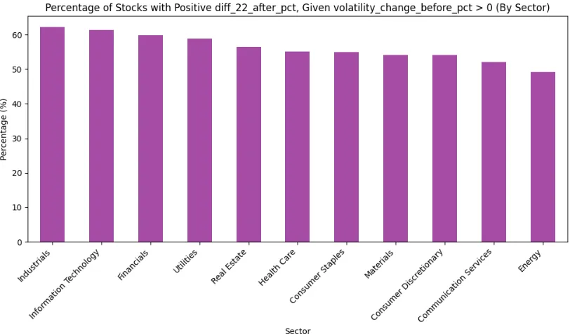
As we can see from the chart, there are no clear differences in the sector. All the sectors, when they were volatile before the announcement, increased their prices by more than 50%, except for one, energy, which is right below 50%.
And what about volume?
# Filter data where volume_change_pct_before > 0
filtered_volume_data = df[df['volume_change_pct_before'] > 0]

# Group by sector and calculate the percentage of diff_22_after_pct > 0
sector_diff_22_positive_pct = filtered_volume_data.groupby('sector')['diff_22_after_pct'].apply(lambda x: (x > 0).mean() * 100)

# Plot the percentages
plt.figure(figsize=(10,6))
sector_diff_22_positive_pct.sort_values(ascending=False).plot(kind='bar', color='blue')
plt.title('Percentage of Stocks with diff_22_after_pct > 0 (Volume Change > 0), Grouped by Sector')
plt.ylabel('Percentage (%)')
plt.xlabel('Sector')
plt.xticks(rotation=45)
plt.tight_layout()
plt.show()

The chart for the volume, looks extremely similar to the volatile one, just with an altered order. Nothing new!
Do the “cheap” stocks behave better?
The stocks whose PE_TTM is under 15, can be considered as undervalued with the potential to grow. Will this affect the results? Let’s plot some of the filters above to see if undervalued stocks will behave better
# First, create filtered dataframes based on the specified conditions
filter_1 = df[(df['consecutive_increase_of_EPS'] > 2) &
              (df['estimated_greater_than_previous_actual'])]

filter_2 = df[df['volume_change_pct_before'] > 0]

filter_3 = df[df['volatility_change_before_pct'] > 0]

# Function to calculate percentage of diff_22_after_pct > 0
def calculate_percentage_diff_22_after_positive(filtered_df):
    total = len(filtered_df)
    positive = len(filtered_df[filtered_df['stock-to-benchmark_22_after'] > 0])
    if total > 0:
        percentage_positive = (positive / total) * 100
    else:
        percentage_positive = 0
    return percentage_positive, 100 - percentage_positive

# Get the percentages for each filter
percentage_1 = calculate_percentage_diff_22_after_positive(filter_1)
percentage_2 = calculate_percentage_diff_22_after_positive(filter_2)
percentage_3 = calculate_percentage_diff_22_after_positive(filter_3)
percentage_full = calculate_percentage_diff_22_after_positive(df)

# Plot the pie charts as subplots
fig, axes = plt.subplots(1, 4, figsize=(10, 10))

# Titles for each filter
titles = [
    'Growth',
    'Volume',
    'Volatility',
    'Full Dataset'
]

# Plot each pie chart
percentages_list = [percentage_1, percentage_2, percentage_3, percentage_full]

for ax, percentages, title in zip(axes.flatten(), percentages_list, titles):
    ax.pie([percentages[0], percentages[1]], labels=['Positive', 'Negative'], autopct='%1.1f%%')
    ax.set_title(title)

plt.tight_layout()
plt.show()

If we run the same code including all stocks, then we will get:

The pie is similar. We see some rationale that the positive behavior is slightly better for the undervalued stocks than the full dataset, but it is so very small (0.3%) that cannot be considered as a pattern.
Conclusions
Even though the results are quite balanced, and no strategy can work solely on those, there are some key takeaways to have in mind during the earning season.
Earnings surprises: Analysts are typically conservative, but even small positive surprises tend to have a balanced effect on stock prices before and after earnings announcements.
Sector behavior: Certain sectors like Utilities and Communication Services tend to benefit more from positive surprises and constant growth, while others like Materials show irrational behavior, sometimes reacting positively to negative surprises.
Pre-announcement volume and volatility: Increased volatility and volume before an announcement generally lead to a positive post-announcement price action, but there are no strong sector-specific patterns.
Undervalued stocks: Stocks with a Price-to-Earnings ratio below 15 perform slightly better than the broader dataset, but the difference is marginal and not indicative of a clear trend.
Growth stocks: Stocks with consistent earnings growth (three or more consecutive quarters of increased EPS) exhibit mild positive price trends starting a month before earnings and continuing for two weeks after, though the pattern is not strongly significant.
With that being said, you’ve reached the end of the article. I hope you learned something new and useful today. As always, I’m open to constructive criticism. So pour your thoughts and suggestions in the comments. Thank you for your time.
Disclaimer: While we explore the exciting world of investing in this article, it’s crucial to note that the information provided is for educational purposes only. I’m not a financial advisor, and the content here doesn’t constitute financial advice. Always do your research and consider consulting with a professional before making any investment decisions.
Comentarios